PostgreSQL Stories: From slow query to fast—via stats

You might have heard “it’s important to know your data” when working with databases. But what does that look like in practice? This post is one answer: an example of how knowing our data helped us debug a slow query. This is Part 2 of a longer story. In Part 1, we discovered what was blocking Render’s staging deployment pipeline. The culprit was a simple query that was taking hours to run against our staging PostgreSQL database: At the end of Part 1, we hadn’t yet figured out a big mystery: why was this query taking so long? It looked so simple. Here in Part 2, we dive into how we pinpointed and fixed the root cause of the slowness. Along the way, you’ll see many database tools and concepts in action, such as:

• EXPLAIN: a command that returns the steps a database will take to execute a query.
• Join algorithms: the algorithms a database uses internally to join two sets of data. These algorithms include merge join, hash join, and nested loop join.
• PEV2: An open source tool that visualizes PostgreSQL execution plans.

A quick gut check

Let’s pick up where we left off. After taking a moment to celebrate finding the culprit query, we dove into figuring out what was wrong with it. We started with a quick temperature check. The query passed this test:

• It’s simple. The query joins two tables on a straightforward condition. It does not pull from dozens of tables nor re-aggregate data.
• It’s indexed. There’s a relevant index on each table in the query: The postgres_dbs table has a unique btree index defined over postgres_dbs(database_id). The events table has a multi-column btree index defined over ((data ->> 'serviceId'::text), "timestamp").
• It’s bounded. The LIMIT 1 ensures PostgreSQL won’t send back every event. The query will stop executing after one match.

There were no obvious red flags here, so we moved on to deeper diagnostics.

Needles in a haystack

To get a sense of the scale of the data we were working with—which, as a reminder, was in our relatively small staging database—we ran a few COUNT queries over the two tables in question. We found that:

• The postgres_dbs table contained ~100k rows.
• The events table contained ~90M rows.
• Only up to ~10k rows in events (0.01% of events) were associated with a row in the postgres_dbs table.
  • Note: This was a rough count. We counted all events that had a prefix (dpg-) that indicated they were associated with postgres_dbs.

As the numbers show, we had a “needle in a haystack” problem: only a small fraction of rows in one table (events) could be joined with a row in the other table (postgres_dbs). This is a classic type of problem that, in theory, a well-indexed relational database solves.

Query plan: using EXPLAIN

Next, we issued an EXPLAIN. We wanted to know how the database was executing our query: An EXPLAIN returns a “query plan”: a description of the algorithm the database will use to fetch the results for a query. Each step of the algorithm is returned with the estimated “cost” of that step. The higher the cost, the longer a step takes to run. Note that there’s a variant of EXPLAIN called EXPLAIN ANALYZE. EXPLAIN ANALYZE gives a more accurate measure of cost. Instead of providing an estimate, it actually runs the given query and returns real “costs”. Unfortunately, we couldn’t use EXPLAIN ANALYZE because our query was taking hours to run, and we didn’t want to wait. So we ran the basic EXPLAIN. Here’s what we saw: This query plan looks reasonable. Here’s a quick explanation:

• The two most indented lines (Index Scan… and Index Only Scan…) are executed first. These two lines indicate the database will access the events and postgres_dbs tables with the indexes we mentioned above (events_service_id_timestamp_idx and postgres_dbs_database_id_key). The events will be scanned in order by serviceId, and the postgres_dbs in order by database_id.
• PostgreSQL will use a merge join to join the two datasets.
• The outer Limit […] rows=1 in the query plan indicates the merge join halts as soon as one row is joined.

Aside: What’s a merge join?

A merge join works like this. First, picture two columns of data, each in ascending order. Each column has many rows. Now:

1. Initialize a pointer i at the beginning of one column.
2. Initialize a pointer j at the beginning of the second column.
3. Until either i and j exceed the bounds of their columns, repeat the following:
   1. If the values of the ith row and the jth row match, emit a joined row.
   2. Else, if the value of the ith row is “less than” the value of the jth row, advance the i pointer to the next row.
   3. Else, advance j.

Merge joins can be an effective strategy when two sets of data are already sorted.

Houston, we’re scanning too many rows…

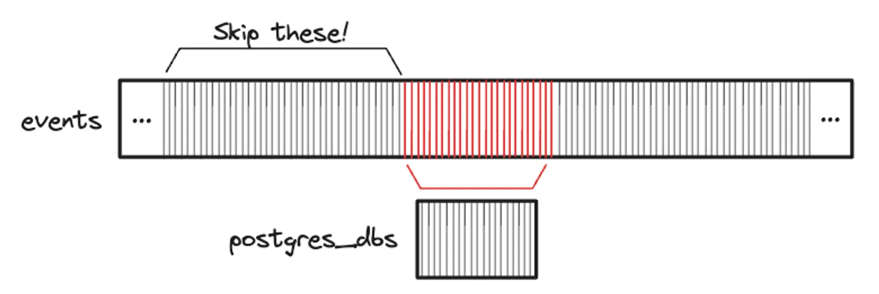
After getting the query plan, we stepped back to think about what was going on. We decided to draw a conceptual picture of the merge join. In drawing our picture, we wanted to reflect the following facts about our data:

• As noted above, only a small fraction of events (0.01%) are related to a postgres_db. The majority of events are related to other things—for instance cronjob runs, server builds, user logins, and other events on the Render platform.
• The serviceIds in the events table are prefixed based on the event type. For example, serviceIds for cron jobs start with crn-; serviceIds for PostgreSQL databases (represented by rows in postgres_dbs) start with dpg-; serviceIds for servers start with srv-; and so on.
• The index on the events table is sorted by serviceId.

Our picture of the merge join looked like this:

A light bulb went off. Our picture helped us see that the database would first scan through all events that appear earlier in sort order than events related to a PostgreSQL database (dpg-). Thus, the query was likely taking a long time because it was first scanning through a huge number of events that would never join to a row in postgres_dbs. To understand just how many other events had to be scanned before we reached events for a PostgreSQL database (dpg-), we ran a few more COUNT queries. We saw that:

• 79M of the 90M events (87% of events) appeared in alphabetical order before events associated with a PostgreSQL database. These included a large number of cron job events (with prefix crn-), which occur frequently.
• Of the remaining ~11M events:
  • ~10k events were associated with a PostgreSQL database.
  • ~10M events appeared in alphabetical order after PostgreSQL database events. These included server events (with prefix srv-).
  • ~600k events had a null serviceId. By default, NULLs are ordered after non-null content in PostgreSQL databases.

Manual fix 1: Skip earlier rows

We now understood the slowness. But, how would we fix it? We wanted our query to skip all the events at the start of the index that would not match.

So, we added a WHERE clause to our original query to force PostgreSQL to jump to the relevant events: This new query returned a result in less than 2ms. Awesome! Problem solved?

Unchanged query plan

We’d just crafted a query that would finish running in a reasonable time—2ms—so we could now issue an EXPLAIN ANALYZE to get more details about the query execution. We visualized the result via the PEV2 tool hosted by Dalibo:

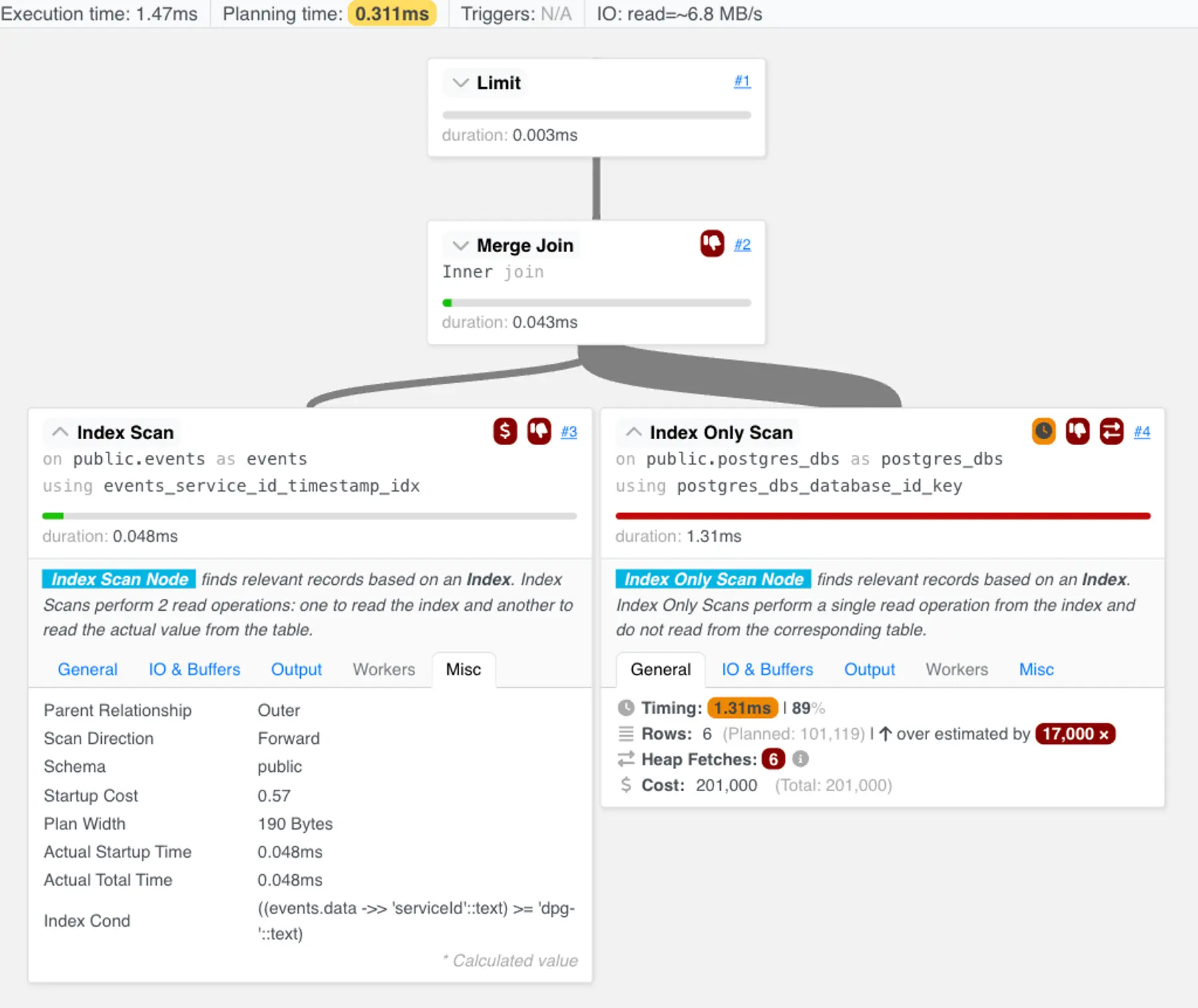
The new query plan looks similar to the original query plan. The only difference is a new index condition that reflects the WHERE clause we added. Though we had a working solution, something about it felt off.

The “full” query yields a surprise

To further investigate, we decided to try to fetch all matching rows, instead of just one. We reissued the query without the LIMIT (let’s call this the “full” query): Here’s what we guessed would happen:

• We expected all matches to return quickly. As you recall, there were only ~10k rows in the events table associated with a postgres_db row, and therefore at most 10k rows in the full result. That is a tiny number of rows for a computer in the 21st century.
• We expected the query plan to look similar. We expected the plan to also use a merge join. This time, we expected the merge join to keep joining records until we hit the end of the index on postgres_dbs.

Here’s what actually happened: to our surprise, the query took two and a half minutes to run, and the query plan looked very different.

Analyzing the “full” query

We ran EXPLAIN ANALYZE on the “full” query, and visualized the result.

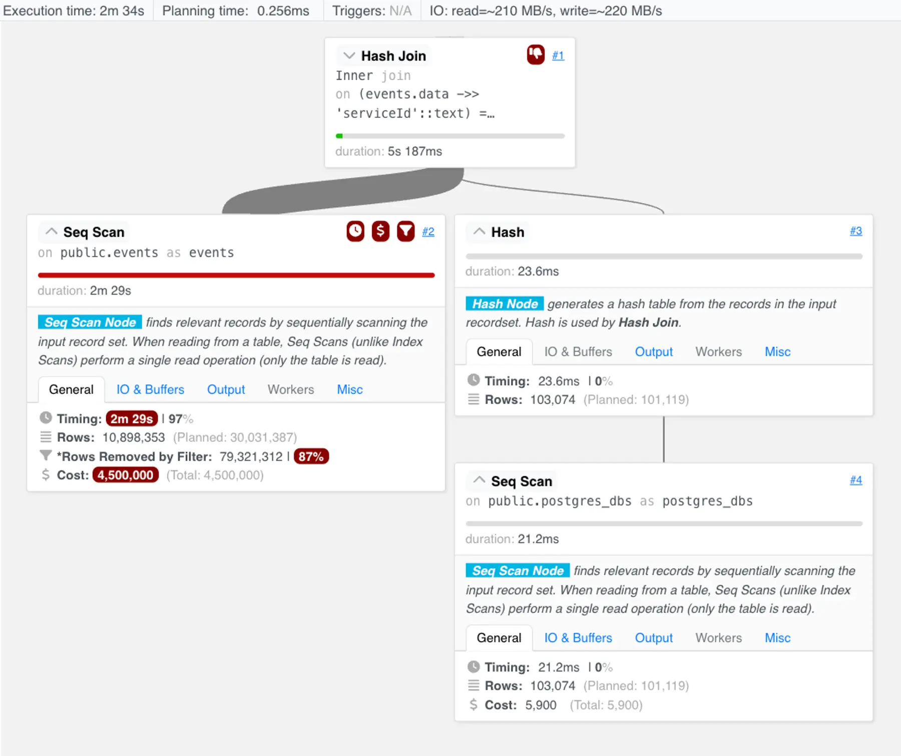
We saw that a hash join was chosen instead of a merge join. This can be an effective choice when one side of the relation is much smaller than the other—which is the case here.

How the hash join works

As this query plan shows, the hash join is executed as follows:

1. First, the whole postgres_dbs table is scanned. Each row is inserted into a hash table keyed by the row’s database_id. This hash map is constructed in ~23ms.
   • Note: Since we're consuming the entire postgres_dbs table, a sequential scan isn’t alarming. Using an index may be slower: an index scan would select rows from the index and then fetch them from the table, which is more work than just scanning the table.
2. Then, the hash table is probed for a matching entry for each row in events.

Unfortunately, the query planner goes off the rails in step two. It chooses to do a sequential scan over the events table. The planner had regressed back to churning through many rows of events that would never join with postgres_dbs.

Manual fix 2: Skip end rows

Ideally, we wanted to replace the sequential scan over the events table with the same index scan from the previous plan. That would let us skip over the many rows we end up filtering out. We thought of several way to get PostgreSQL to do this—some better, some worse:

• We could rewrite the query with a materialized CTE that would first scan the relevant events and store them as a temporary table for a subsequent join. However, this is a heavy-handed approach. We're also likely to spill to shared memory and disk to store a large intermediate result set.
• We could introduce an ORDER BY <expression> to the query, and hope that the query planner opts to scan an index that is ordered by the same expression.
• We could be more explicit in telling PostgreSQL what our data distribution looks like. Earlier, we added a condition to skip the events that occur before a database-related event in an index scan. This leaves the tail of the index starting at database events, but still includes ~11M events that won't match the join condition.

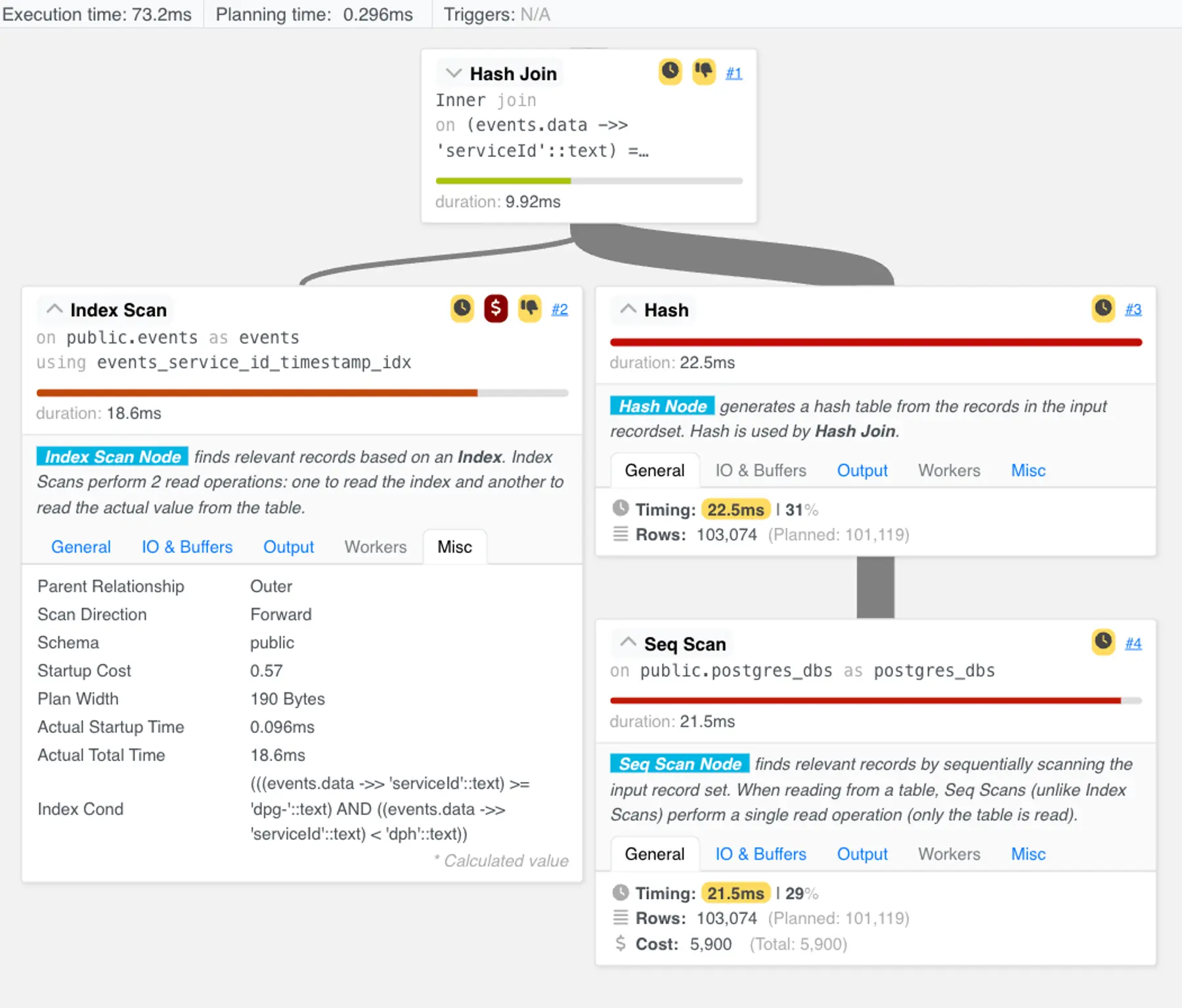
We decided to try the third option:

This query returned all the events for databases in about 70ms. Finally, we had achieved the kind of speed we expected for this query. An EXPLAIN ANALYZE showed that the new query plan looked as we expected. The sequential scan was replaced by an index scan that finished in under 20ms:

At this point, we could have declared success. If we had only wanted to fix the slow query, we’d be done.

A statistics lesson

But we wanted more—we wanted to understand the root problem. In our experience, PostgreSQL’s query planner should be able to pick the optimal plan for a query like this, without the WHERE clauses. Why wasn’t PostgreSQL making the right choices right now? We began to suspect our PostgreSQL instance “knew” less about our data than we thought it did.

Aside: What are “statistics” in PostgreSQL?

In the background, PostgreSQL instances automatically gather a number of statistics about the data within each table. Statistics include things like:

• the number of rows in a table
• the physical size of a table or index
• the distribution of data in each column of a table

PostgreSQL instances use statistics to estimate the cost of different query plans. You can query these statistics via the pg_stats view. PostgreSQL periodically updates these statistics as a table changes. You can also manually trigger an update by running ANALYZE.

Querying our statistics

We queried the statistics for the data column of the events table: (Note: Columns are clipped and reformatted for readability.) Here’s what each statistic means:

• null_frac: the ratio of null rows to the total number of rows. In the above output, the value 0 means there are no null rows.
• n_distinct: either the absolute number of distinct values in a column (indicated by a positive number), or the ratio of distinct values to the total number of rows (indicated by a negative number). In the above output, the value -0.22765513 means that 22.7% of rows contain a distinct value.
• most_common_vals and most_common_freqs: a list of the most common values. In the above output, we (unfortunately) see many events related to server and cronjob crashes.
• histogram_bounds: a sampling of every nth element when the column is sorted. These bounds break the rows of a column into groups of roughly the same size. These bounds can be used to estimate the cardinality of a result.

We noticed right away what the problem was: the format of each “value” (as seen in the most_common_vals column) in these statistics did not match the format needed to determine the right query plan for the (e.data -->> 'serviceId') expression. Thus, the query planner was unable to make use of these counts and frequencies, and was basically doing the best it can with default assumptions. Instead of statistics on the JSON objects we saw in most_common_vals, we wanted statistics on just the serviceIds. Now we knew exactly what to fix.

Ultimate fix: DIY stats

PostgreSQL lets you create statistics, explicitly. Creating statistics is a powerful tool to boost database performance. While we won’t dive into full details here, know that you can empower the query planner with information like:

• Which columns are heavily correlated with one another (e.g., a postal code will always belong to a specific city)
• Which columns can predict the value of another (e.g., if a user id uniquely determines an email address, and vice versa)
• Statistics over expressions that are useful for you to filter or sort by (e.g., keeping a histogram of price * exchange_rate)

In our case, we wanted to track statistics on the serviceId of each event. We ran this query to create the statistic: Once these statistics were populated, we queried them via the pg_stats_ext view: Compared to the statistics we saw before, there are notable differences:

• null_frac: There is a non-zero proportion of NULL values.
• n_distinct: The number of distinct values is positive, which indicates an absolute count of distinct values.
• most_common_vals: The values here are serviceIds, which is what we want to filter by in our original query.

Final test and query plan

It was now time to test the impact of adding these statistics. We re-issued our original query—the one that had hung for hours. It finished in a fraction of a millisecond! We looked at the new query plan:

Notably, this plan now uses the most vanilla of join types: the sturdy nested loop join. This join algorithm takes one row from the left relation, and queries all of the rows in the right relation that match the join condition. For this particular query, it's a great plan, because most postgres_dbs will have at least one event associated with it, and the index lookup is a very fast way to find the set of events for a particular database. For completeness, we once again removed the LIMIT in the original query and tried fetching the “full” results:

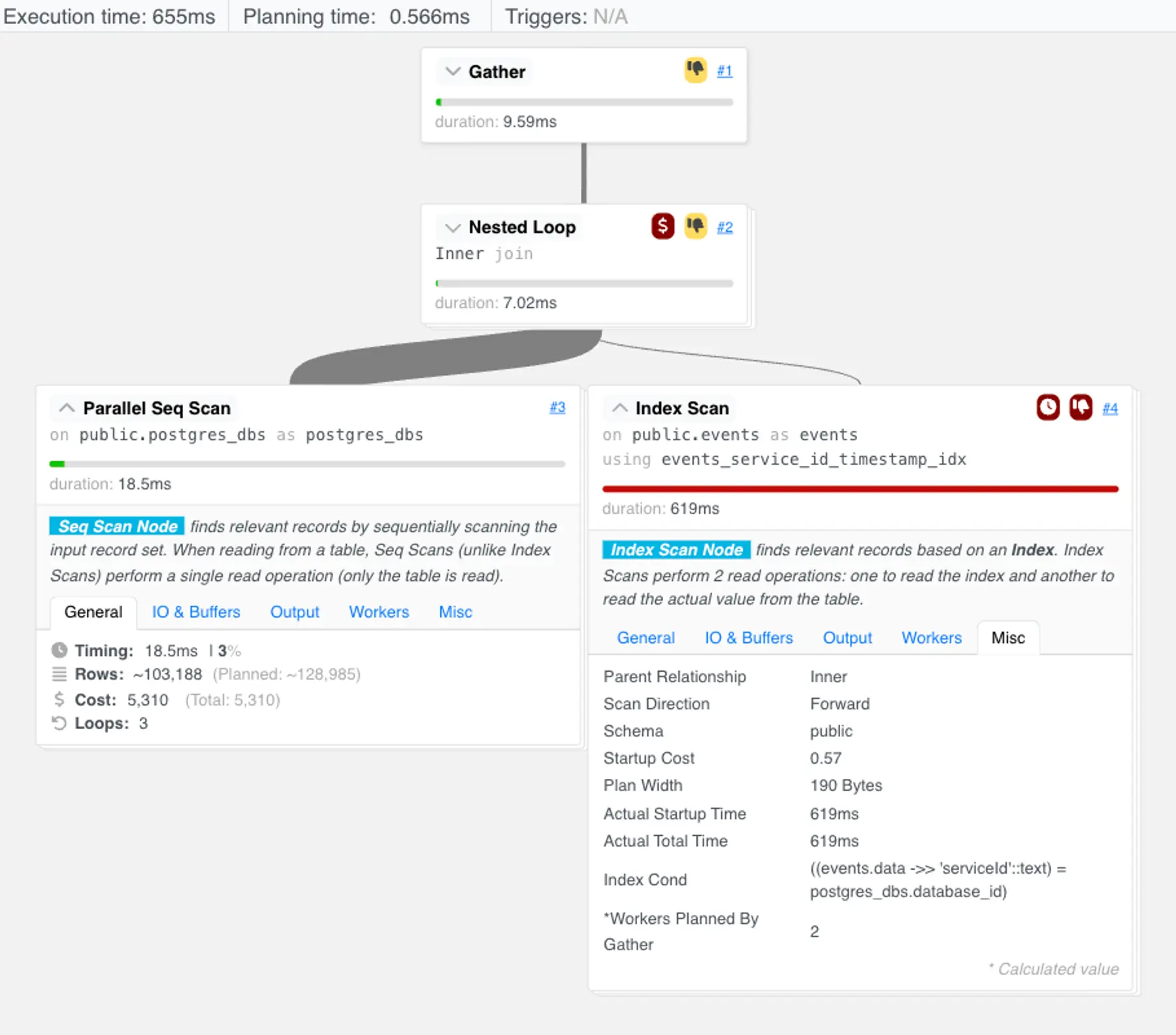
PostgreSQL kept a very similar query plan and returned the ~10k result set in about 650ms. Now that was the kind of performance we expected. QED.

Tools for you

The tools we mentioned in this story can help you in a similar situation. Try out the techniques you just saw:

• Run EXPLAIN or EXPLAIN ANALYZE on a query. Remember that EXPLAIN ANALYZE actually executes the query.
• Use the PEV2 tool to visualize an EXPLAIN ANALYZE run.
• Explore the pg_stats view in your database.

You can find all of these commands and more in our PostgreSQL performance troubleshooting guide. Bookmark it for the next time you’re debugging slowness or optimizing a query.